 |
|||||||
|
|||||||
Simulation of Sonar Beampattern
|
|||||||
| This page gives a short introduction of how the simulations were done and a comparison of simulated and measured beampattern for a given transducer. | |||||||
|
The Simulation Principle
The calculations shown here base on the same principle as the calculations of the diffraction pattern of optical instruments that can be found here (under construction). We have an array that is the source of a plane wave, in the case of the sonar array we have the sides of the transducers that face the water. On the physical basis of interference and diffraction of acoustical waves the geometrical arrangement of the sound projecting plane determines the pattern of sound that is sent away from the transducer. The basis of the simulation is always this geometrical arrangement, the result of the simulation, the soundfield or beampattern of the transducer, is shown as a two-dimensional grayscale image or as a polar plot. The simulations are valid for the farfield only, corresponding to Fraunhofer Diffraction. This means for instance, that for a transducer 500mm long working at 50kHz the simulated beampattern is valid at all distances larger than 5 meter from the transducer away. Any curvature of the sound projecting plane of the transducer can not be considered up to now. The sound projecting plane can have any geometry. It is represented by a bitmap that is shown for each simulation, white color represents areas where sound is emitted. Areas of different intense sound emission can be represented by a grayscale. The program also gives the percentage of energy concentrated in the central lobe. The Program The diffraction simulation program was written by me in Visual C++ because I could not find any product to fit my requirements and for to learn programming with C++. Originally it was a program to simulate diffraction pattern of optical instruments, but, inspired by the need to work with ultrasound generation in my daily job I added the functionality to simulate sonar and other wavefields as well. Dynamic All soundfields are calculated down to -25dB. Professional measured polar plots in many cases go down to -50dB, but the plots calculated for -50dB turned out to be relatively confused because of many small sidelobes. Since the sidelobes smaller than -25dB can be neglected in practice I decided to display the beampattern down to -25dB, the only exception are the simulations shown on this page for the reason to be comparable with the measurements. Frequency I have chosen 50kHz instead of 200kHz for most of the simulations, since this is the frequency where you would preferentially like to run the fishfinder transducer arrays, since they will give a vertical beamwith of 45° at -3dB for 50kHz that is good to work with, but a narrow 11° at 200kHz, that would be very problematic to find the correct combination of downtild angle and hight above ground for a reasonable range. |
|||||||
|
Can
we trust the results?
This may be one of the first questions that arises, so I simulated some existing transducers and compared the simulated beampattern with measured ones I found in publications. In the following I will present the results for the transducer model B256 from Airmar Technology Corporation, a commercial fishing 50/200 kHz transducer with an element configuration of four circular elements with 44 mm diameter, arranged in a diamond shaped pattern (Fig. 1). This transducer is of special interest, since it consists of the same or very similar elements most of the 50/200 kHz fishfinder transducers are made of. |
|||||||
|
|||||||
|
|||||||
|
|||||||
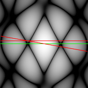
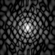
| The
simulated
beampattern (black) in Figures 2 and 3 show a good correspondence with
the measured ones
(green) from the technical datasheet, especially concerning position,
but also the relative intensity of the sidelobes. Below -30dB the
correspondance gets worse, this may be a result of internal
reflections and absorbtions in the real transducer that are not
included in the
simulation. This is one more reason for my decision to display the
other simulations only down to -25dB. The small sidelobes at +/-
20° that are present in the 50kHz measured pattern are
completely absent in the simulation. This may also be a result of
internal
reflections - or, as can be suspected when viewing the two-dimensional
maps of the 50kHz beampattern (Fig.4a), are a result of a small tilt
of the transducer during the measurement. If the polar plot in Figure 2
does not
represent a section along the green line in Fig.4a, but along one of
the red
lines small sidelobes at +/- 20° will appear. They will also
appear, when the listening hydrophone for the measurement covers an
angle of more than 6 degrees. |
|||||||
|
|||||||
|
|||||||
|
At
angles larger
than +/- 75° the simulations often show strong deviations from
the measured beampattern, this may be a result of the fact that the
simulated transducer have no sound absorbing enclosure from the back
and the sides as real ones and no housing to alter the pattern. For
this reason I run the simulations only to angles of +/-
80° in most cases.
|
|||||||
| |